Double Fourier Series

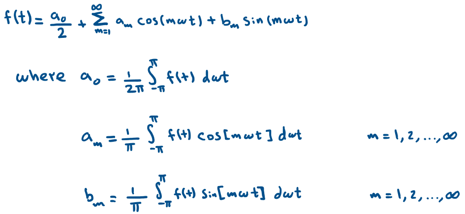
Joseph Fourier “invented” his famous, ingenious, and whats considered by many engineers as the most useful equation in their toolkit. However, the original Fourier series is concerned only with an equation of one variable dependency (often as a time variable).
But what happens when we have a function that depends on TWO Variables to be formulated? How can we then tweak the original Fourier formula to account for this new situation? In fact, the function we are referring to is the ubiquitous PWM function that is used in almost any electronic device.

---

This article dose not explain the basics of Fourier Series, if you are unfamiliar to it or need a refreshment, I highly recommend the 3Blue1Brown video on it.

---

In the case of PWM functions, we have f(t) that depends on other functions V_ref(t) and V_c(t) to be generated), HOW do we represent such a function as Fourier series that accounts for all variations of V_ref(t) and V_c(t) ??

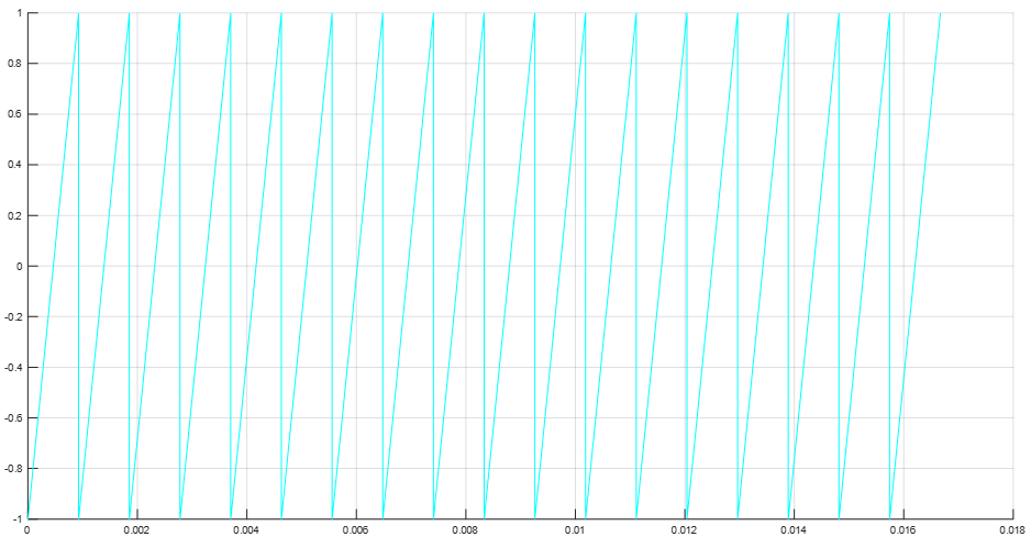
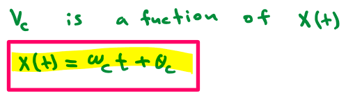
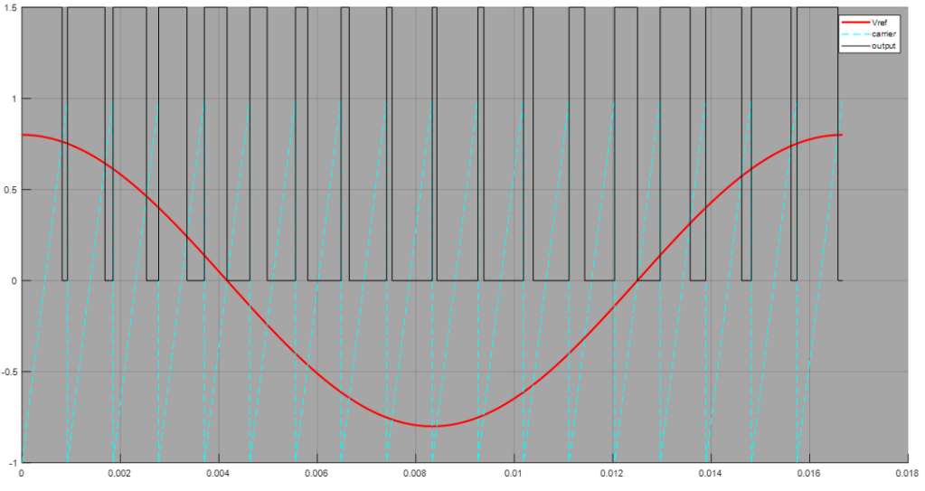
Let V_c(t) be a sawtooth wave (which is a common choice for any converter pwm)

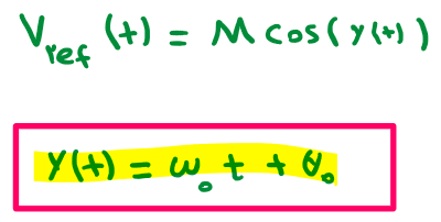
and let V_ref(t) be a sinusoidal function which we will reference to modulate the output to resemble.

and let f(t) ={ 1.5 if V_ref(t) > V_c(t) or 0 otherwise }

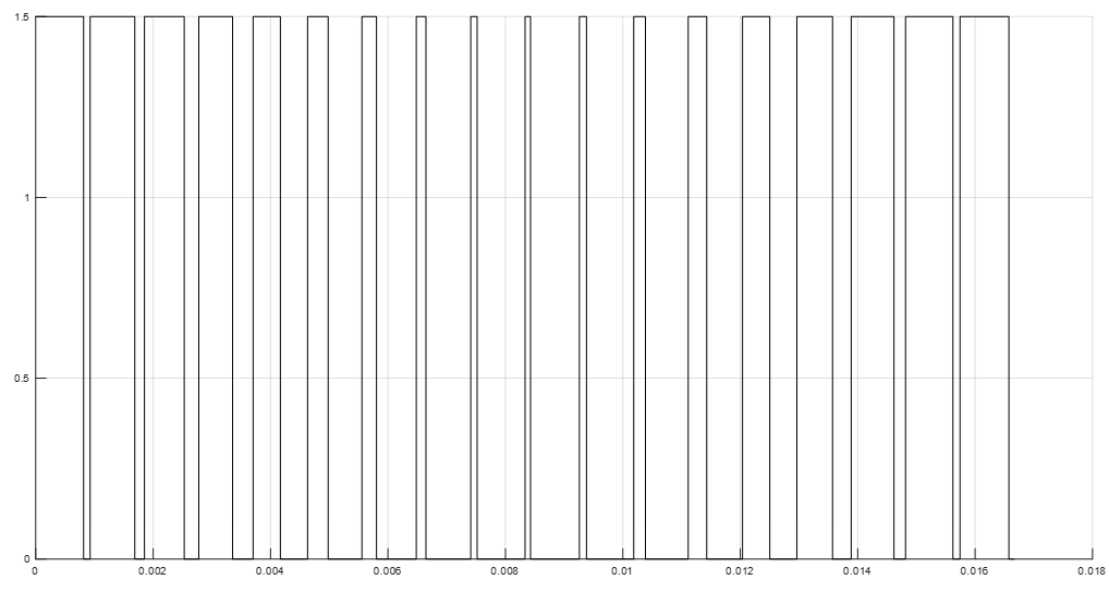
Putting all the conditions together in one picture we get our good old PWM signal.

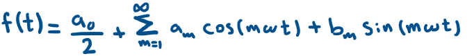
Now, if we want to represent the PWM function f(t) by its comprising harmonic elements, we can simply use the Fourier series.

We can easily_{(well!! it depends on your definition of easy)} do this operation…
HOWEVER, doing so will not yield to any significant insight on how any change on V_ref or V_c would impact the harmonic performance of f(t), and we SHOULD be interested in investigating their correlation since f(t) is a production of the aforementioned signals.

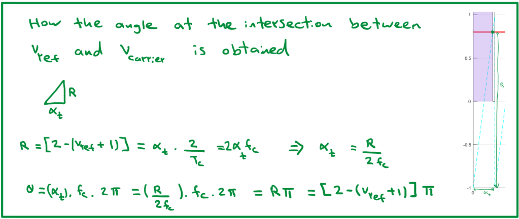
BUT… how do we start? how can we decouple the dependency on the two functions to get the harmonic content?

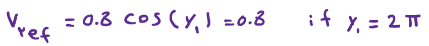
How about we assume that V_ref is constant, we can then chose any point y in V_ref(y) and examine what happens. Let y = 2π then V_ref(y) = 0.8 Cos( 2π ) = 0.8 _{(BTW, 0.8 is the amplitude modulation index of a converter, but that’s a different topic and you don’t need to worry about it for this discussion)}

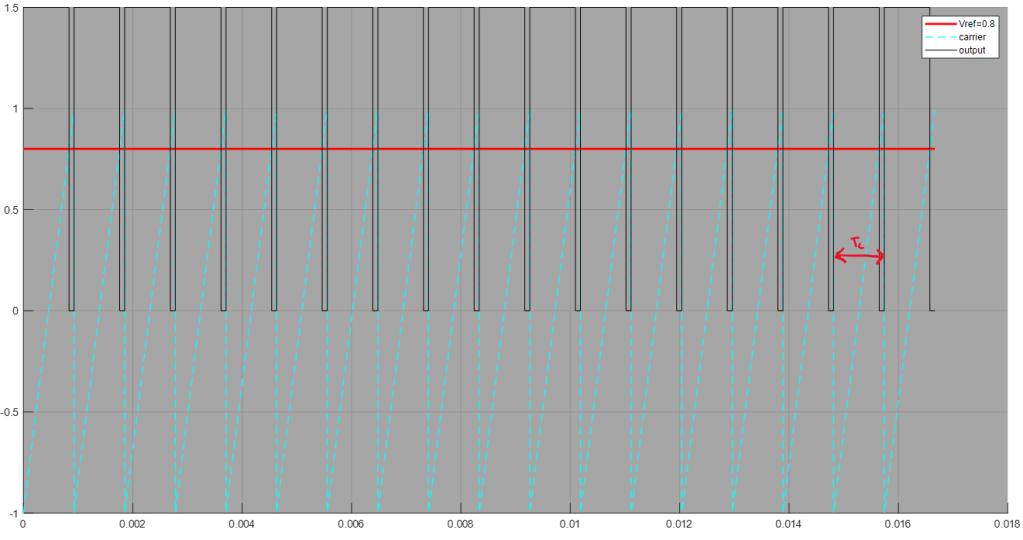
Notice how the frequency of f(t) changed from w₀ -> (which is also the frequency of V_ref) to w_c -> (which is the frequency of V_c)

and if we get the Fourier series of f(t) with a constant y=y₁ it will be:

if we try to calculate the Values of the Fourier coefficients a₀,a_m,b_m for this case when y=y₁ and lets set y₁=0 _{(nothing special about zero, we could’ve chosen any value from the entire span from 0 to 2π)} and observe the Values we get for the coefficients for the first carrier Harmonic.

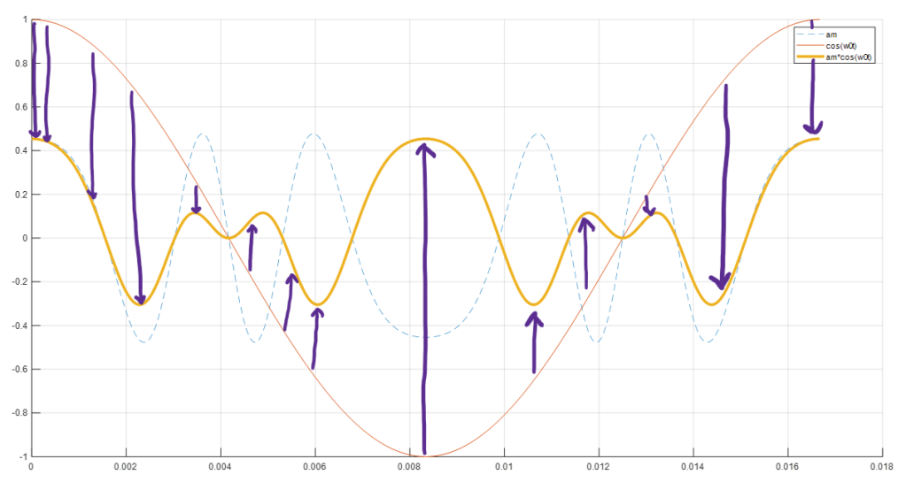
if we try to do the same and calculate the coefficients for different values of y and plot their values we get:

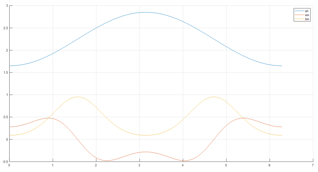
An interesting observation arise, the series coefficients which are normally constant values are turning into cyclic values themselves.
a₀ is clearly a sine wave with a DC offset pushing it upward.
a_m is multiple sine (and/or) cosine waves added together.
b_m is a sine wave of a frequency twice of w_c and a DC offset.

We can highlight some insights from this observation:
– In the first Fourier series we derived for f(t):

the coefficients represent the amplitudes of the sinusoidal harmonic components (Cos(mwt) and sine(mwt)) but if the coefficients themselves are not constant as y changes what would the sinusoidal harmonic components look like?
lets take the term cos(wt)

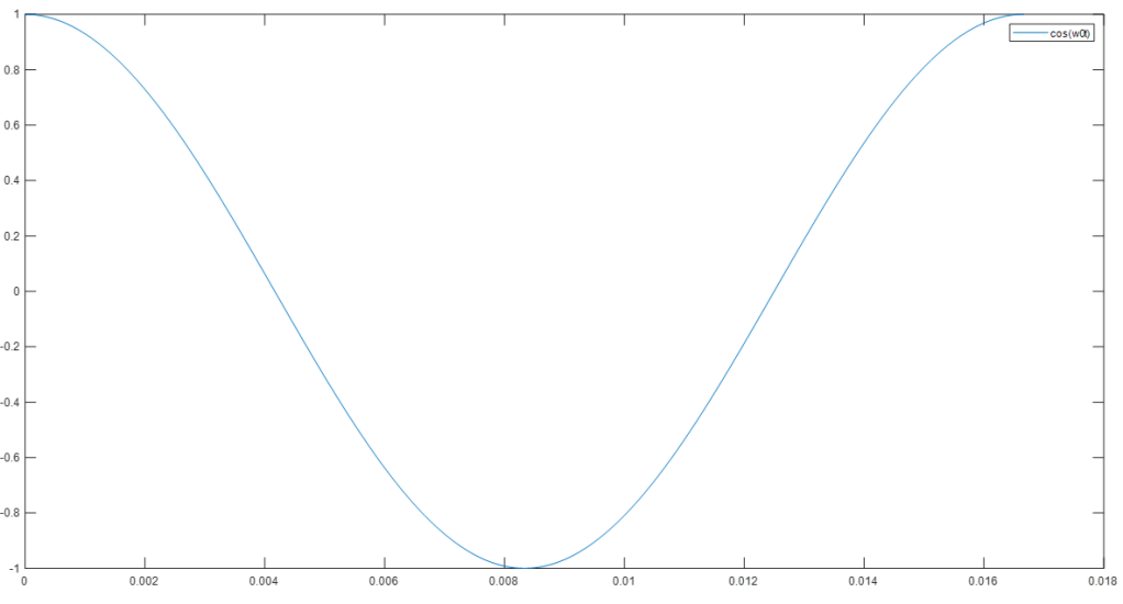
if we multiply a_m to cos(wt) the result should look like:

Thus a_mcos(wt) is also a cyclic function that consists of multiple frequencies

Now if you are asking yourself, “doesn’t this mean that the coefficients can themselves be broken down into a Fourier series of different Harmonic Components???”
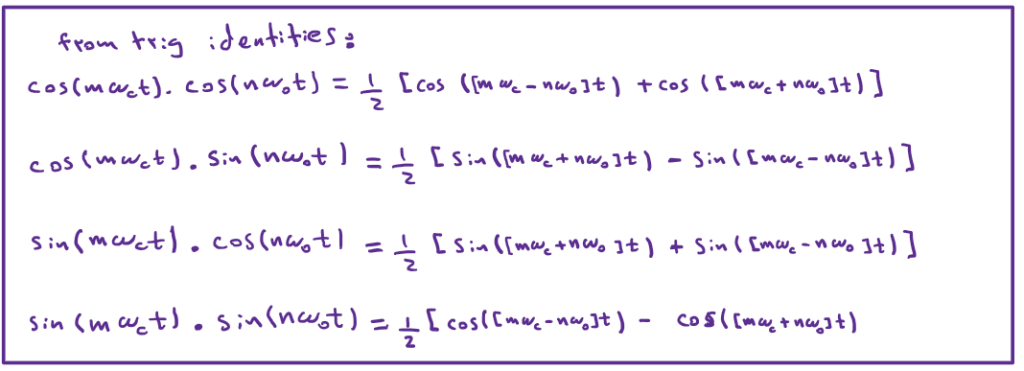
YES indeed, precisely. This is exactly what we should do, we will find the Fourier series of each of the coefficients with respect to y. Then the Fourier components of the the Fourier coefficients (of the “parent” Fourier series) shall be multiplied together and the result of multiplying different sinusoidal functions can be broken down by trig identities.

Ok, I know This sounds daunting But bare with me, it will get clearer as we get there.

Now we need to find the Fourier series for each of the coefficients a₀,a_m,b_m

Similar to what we did earlier, the new Fourier series coefficients have to be calculated to get the amplitudes of the harmonic components of the sinusoidal and DC elements in a₀,a_m, and b_m due to variations in y.

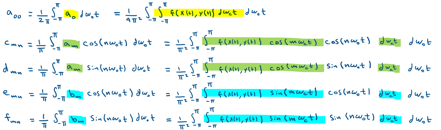
Notice How we get cosine and sine terms of different frequencies (w_c and w₀) multiplied by each others, here comes the trig identity separation part that we talked about earlier.

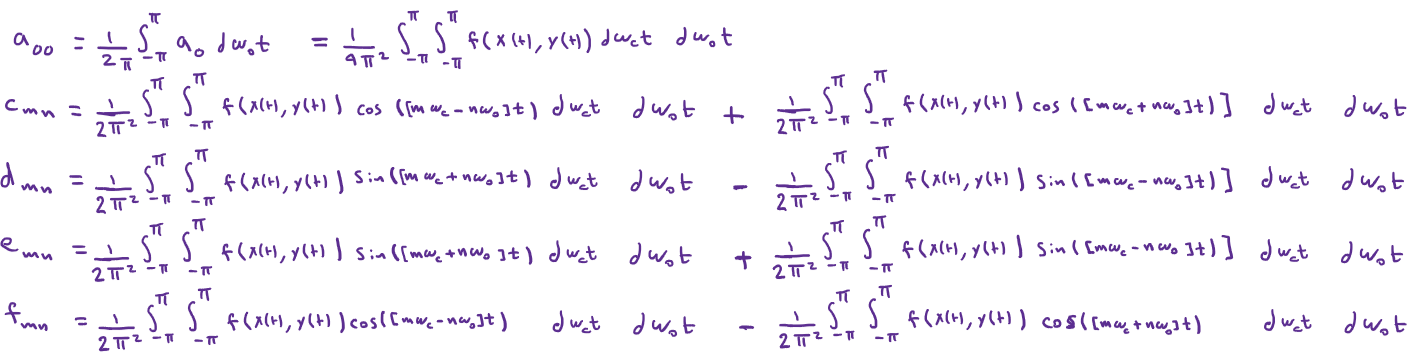
Finally, lets go back to the original equation and plug in the new derived coefficients

Again, we can expand by trig identities to get:

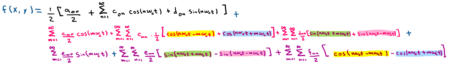
Viola, we are done…

Now we have a beautiful precise analytical expression that can explains where the high carrier harmonic exist and why we have fundamental harmonics as side bands around the carrier harmonics.

In a future post, we shall expand on this derivation to analyze how the choice of the carrier signal impact the harmonic content. It seems that many engineers chose between either the sawtooth or the triangular carriers to perform PWM but they do so without actually investigating the implications and effect of the choice of one carrier or another.

References

D. G. Holmes and T. A. Lipo, Pulse Width Modulation for Power Converters. 2003.